Basic rules allow you to set the format of a column using comparisons to either its own values or another field’s values. This is the most common
...
form of Conditional Format that are applied.
Image Modified
...
Option
Description
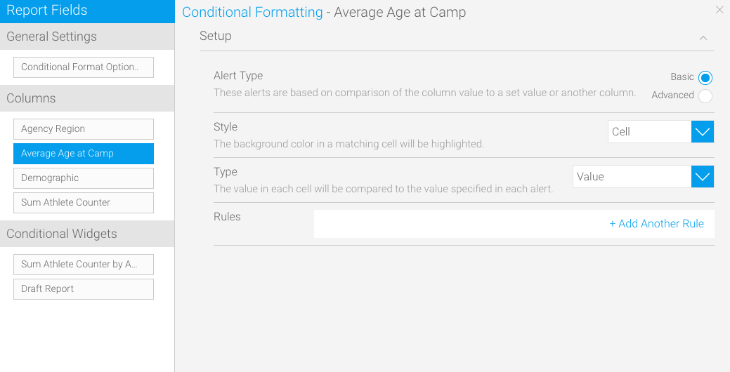
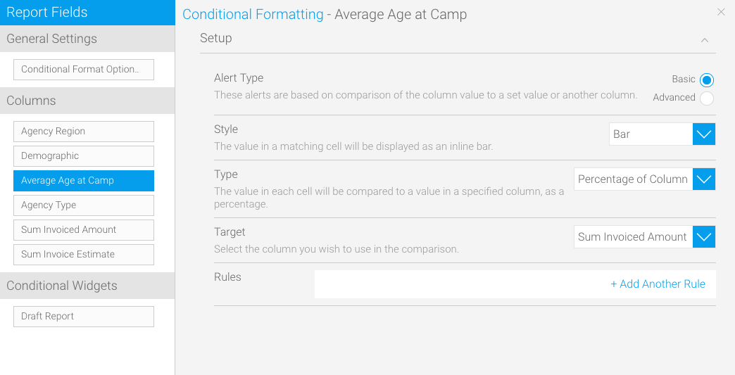
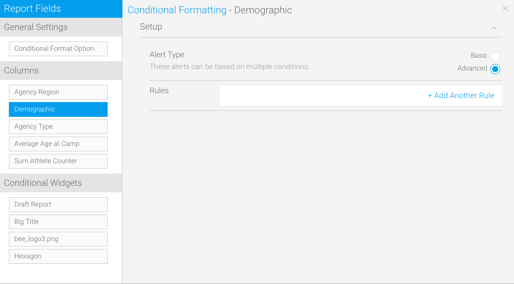
Alert Type
Select the complexity of the alert rules.
Basic: these alerts are based on comparison of the column value to a set value or another column.
Advanced: these alerts can be based on multiple conditions, set up using logic similar to that of Filter Settings.
Style
Select a display method for the alert. There are three options available:
Bar: the value in a matching cell will be displayed as an inline bar. (Note: This type of styling can only be applied to certain types of content.)
Cell: the background colour in a matching cell will be highlighted.
Icon: the text in a matching cell will be replaced with an icon.
Type
Select the comparison type from the following options:
Value: compares data to set values eg. Greater than 10.
Compare Column: compares data to set values stored in another column. E.g. Compare the received amount with amount invoiced to highlight those that are not equal.
Percentage of Column: compares the value to a percentage threshold of a comparison column. Use this to highlight revenue that is 10% less than ‘planned revenue’.
Percentage of Total: compares the value to a percentage of the total of the column. Use this to highlight values that represent less than 5% of revenue.
Percentage of Max: compares the value to a percentage of the maximum value. Use this to highlight values relative to the maximum value eg. values that are in the lowest 20% bracket of results
Target
If you select a column comparison type you will have to choose the column that you want to compare your data to. Choose the appropriate column.
...
Creating Basic Rules on Report Columns
While on the Conditional Formatting popup window, you can create rules with different types of styling. Yellowfin allows users to add three types of styles when rules are matched, as explained below:
Note
Based on the data type of the column, the styling options will differ.
Expand
title
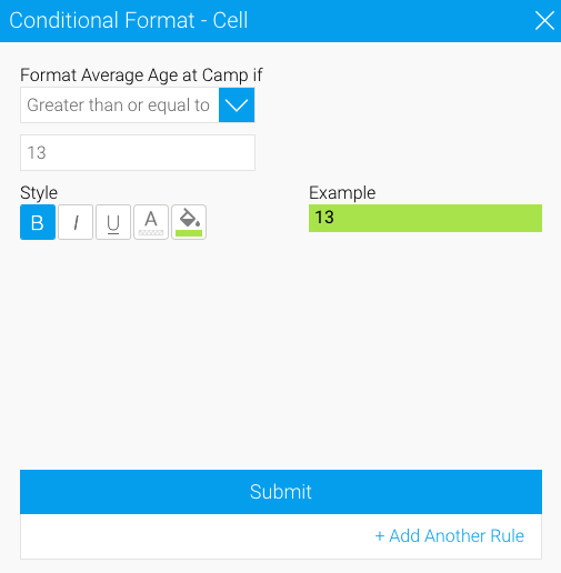
Cell
This can be used to highlight the background colour in a matching cell. For example, you can make it so that if the profits on your monthly report hit a number greater than 500,000, that data will be highlighted with a blue colour.
Follow these steps:
Choose a column from the left side, on which the formatting will be applied
Choose the Basic option from the Alert Type
Select Cell from the Style dropdown
Choose the type of comparison Image Modified
Click on the +Add Another Rule link; a new pop to format matching cells in the report will appear
Start creating a rule by choosing an operator and then adding a value
Set a style to highlight the matching cells
Icon
Style type
Description
Image Modified
Bold
To make the matching values appear bold.
Image Modified
Italic
Make your values italic with this option.
Image Modified
Underline
Add an underline to the matching values.
Image Modified
Font colour
Change the colour of the font.
Image Modified
Background colour
Change the background colour of the matching cell.
Image Modified
Click on the Submit button to save the rule
Expand
title
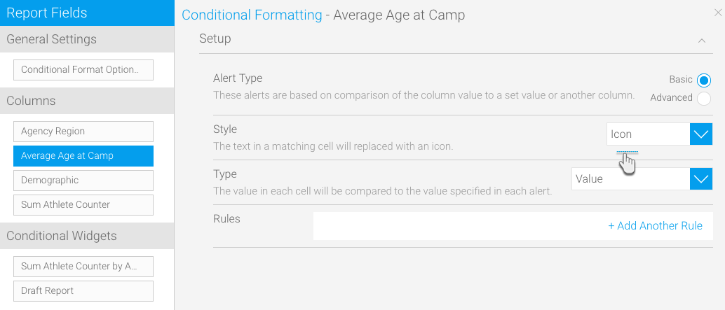
Icon
This can be used to replace the text in a matching cell with an icon.
Follow these steps:
Choose a column from the left side, on which the formatting will be applied
Choose the Basic option from the Alert Type
Select Icon from the Style dropdown
Choose the type of comparison Image Modified
Click on the +Add Another Rule link; a new popup to format matching cells in the report will appear
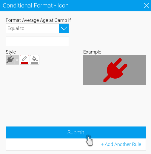
Start creating a rule by choosing an operator and then adding a value
Choose an icon; you can also alter its colours
Icon
Style type
Description
Screenshot
Image Modified
Select icon
Choose from a range of icons
Image Modified
Image Modified
Forefront colour
Change the forefront colour of the icon.
Image Modified
Background colour
Update the background colour of the icon.
Click on the Submit button to save the rule Image Modified
This icon will now appear wherever matched data is found in your report
Expand
title
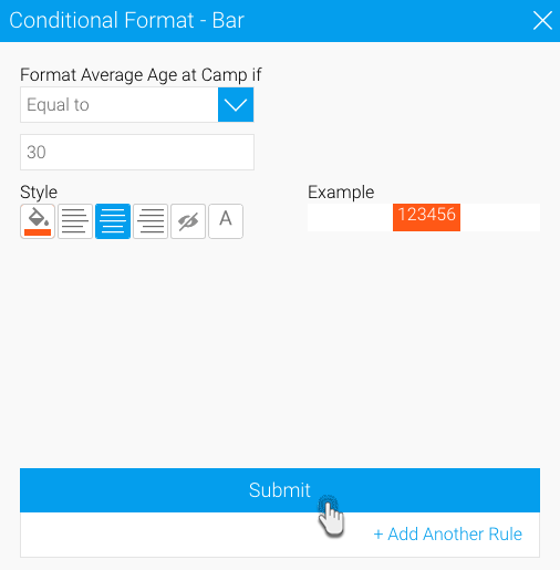
Bar
This is used to make the value in a matching cell display as an inline bar. (Note: This type of styling can only be applied to certain types of content.)
Follow these steps:
Choose a numeric column from the left side, on which the formatting will be applied.
Choose the Basic option from the Alert Type
Select Bar from the Style dropdown
Choose the type of comparison
Select a target value Image Modified
Click on the +Add Another Rule link; a new popup to format matching cells in the report will appear
Start creating a rule by choosing an operator and then adding a value
Style the bar you want to make appear on the matching cells
Icon
Style type
Description
Image Modified
Bar colour
Choose a colour for the bar.
Image Modified
Left alignment
To place the bar on the left part of the matching cells.
Image Modified
Middle alignment
To place the bar in the middle of the matching cells.
Image Modified
Right alignment
To place the bar on the right side of the matching cells. Note: The selected alignment's icon changes to blue
Image Modified
Hide/Show text
Hide or show text/value of the matching data on the bar.
Image Modified
Text colour
If you opt to show text on the bar, you can also change its colour.
Click on the Submit button to save the rule Image Modified
This bar will now appear wherever matched data is found in your report
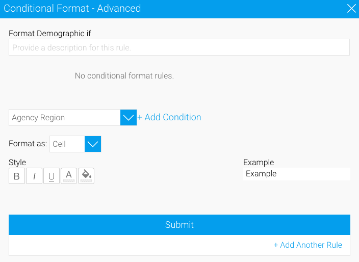
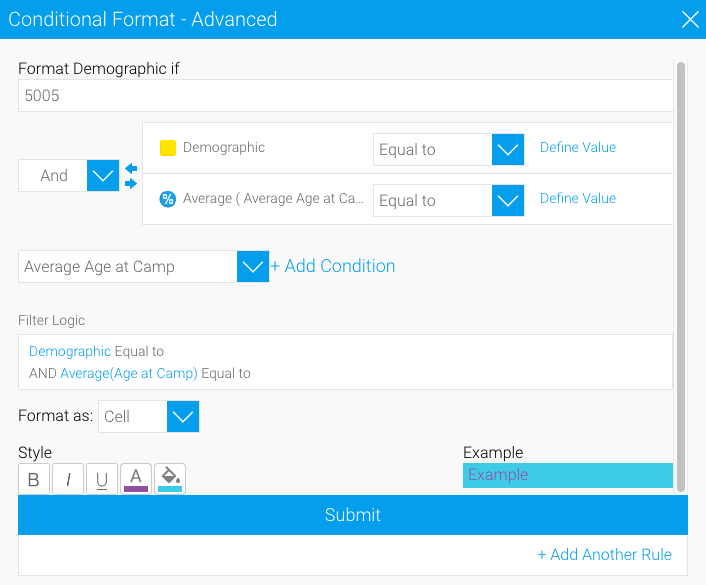
Advanced Formatting
Advanced rules allow you to create complex rules for determining the format of the column. For example, if you wanted to create a rule such as: If Region = Europe and Revenue > $200,000 then highlight Profitability as RED.
Image Modified
Follow these steps:
Choose a column from the left side, on which the formatting will be applied.
Choose the Advanced option from the Alert Type
Click on the +Add Another Rule link; a new popup to format matching cells in the report will appear Image Modified
Enter the logic of your rule. You can select a column the operator and the value. By clicking add you can add additional rules with bracketing etc. See Filter Settings for more information
Choose a format
Style the values the matched conditions will display, the way you want
Icon
Style type
Description
Image Modified
Bold
To make the matching values appear bold.
Image Modified
Italic
Make your values italic with this option.
Image Modified
Underline
Add an underline to the matching values.
Image Modified
Font colour
Change the colour of the font.
Image Modified
Background colour
Change the background colour of the matching cell.
Click on the Submit button to save the advanced rule Image Modified
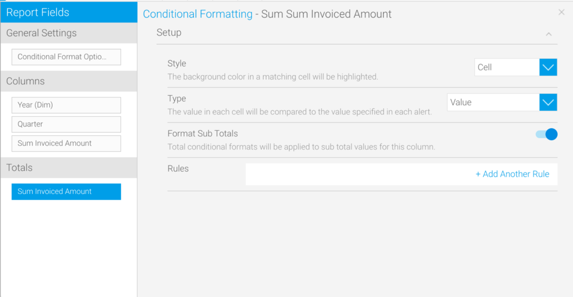
Conditional Formatting on Totals
Image Added
...
Totals
If you have a total value displayed on any of the columns, you can apply formatting rules to those values. The setup configurations for these include:
Option
Description
Style
Select a display method for the formatting rule. There are two options available:
Cell: the background colour in a matching Total cell will be highlighted.
Icon: the text in a matching total cell will be replaced with an icon.
Type
Select the comparison type from the following options:
Value: compares data to set values eg. Greater than 10.
Format Sub Totals
Enable this toggle to apply conditional formatting rules to subtotal cells.
Rule
Create a basic conditional formatting rules, as you would for a Column.