Page History
...
- To set up a Signals analysis, open the relevant view in edit mode. (Note: Cloning a view does not include previously set up Signals analysis.)
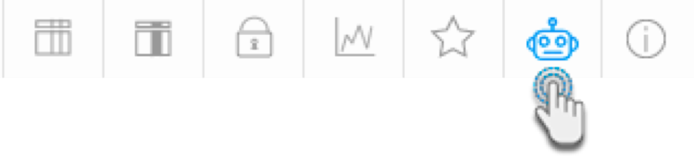
- Navigate to the Prepare page, and click on the automated insights icon.
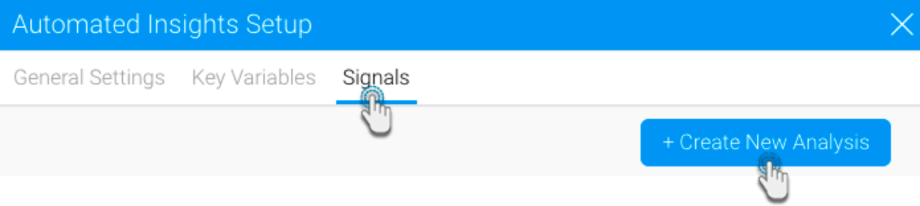
- In the new Automated Insights Setup popup, click on the Signals tab. This will show any Signal analysis that have been created. (If you do not see the Signals tab, ensure that you have the correct role functions enabled.)
- Click on the +Create New Analysis button to create a new Signals analysis. This initiates a multi-step configuration process to help you set up the automated analysis relevant to you.
- Before beginning, establish the type of analysis that you want the system to perform for you. There are three analysis types to choose from. (Refer to the Signals type section here to identify which type of anomaly to detect through one of these analysis types.)
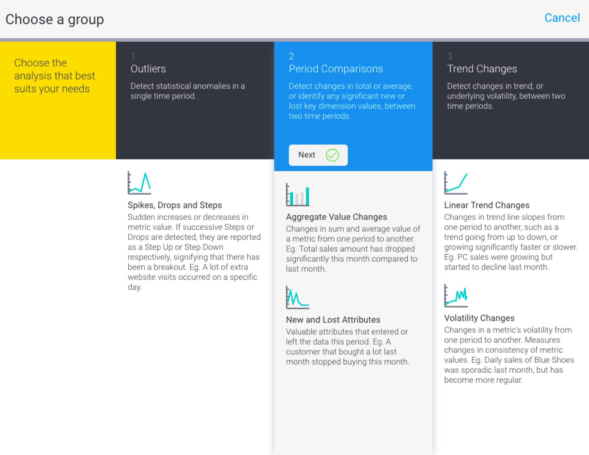
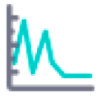
- Outliers - the system detects any anomalies in the data, such as spikes/drops and step changes during a specific time window. These could include rare events, items or observations that are significantly different from the majority of the data.
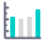
- Period comparisons - identifies changes in total or average between two time periods; and also identifies any significant new or lost key dimension values.
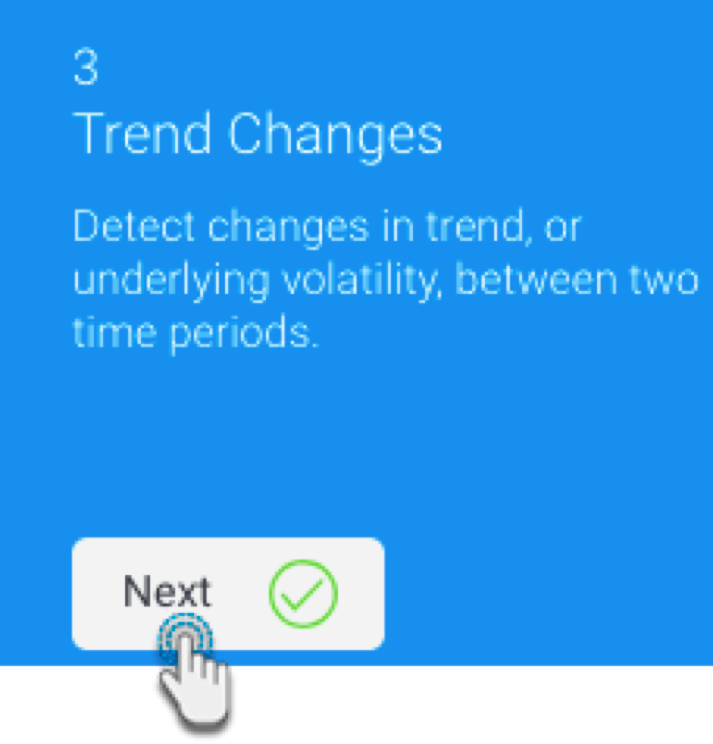
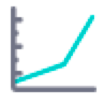
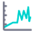
- Trend changes - identifies changes in trend direction between two time periods; and also any changes in the underlying volatility of the data.
- Click on the Next button of the preferred analysis to continue.
In the next step, provide the basic details to describe this Signals analysis.
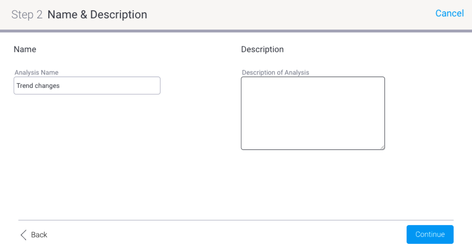
- Name: (mandatory field) A unique name will help you to identify it later.
- Description: Add a description to explain the intent of this analysis.
Continue to the next step.
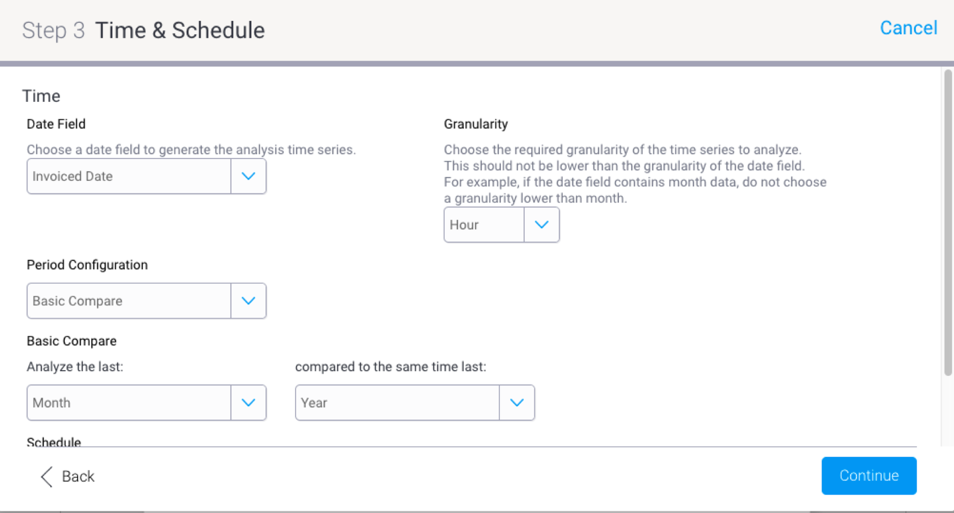
The Time & Schedule step involves highlighting the time periods that you want the system to analyze, along with configuring how frequently this analysis should be executed. Below is a description of each of the settings. (Note: The fields and their purpose differ according to the different analysis types.)
Field
Analysis type
Description
Example
Date field
All
The Signal analysis must include a date field that gets analyzed by the system. This is required to form a time series.
You can choose a date field of any granularity (unit).
Granularity
Outlier detection, Trend changes
Specify the granularity (i.e. date unit) of the time series to analyze.
This value should not be lower than the unit of your selected date field.
For example, if you have a date field with day, then your granularity must be Day or a higher value (Month, Quarter, etc.)
Period comparison
Not required for Period Comparison.he ; the granularity is set to be equal to the window size by default.
Period Configuration
All
This selection changes the time window selection fields. Options are:
- Basic compare: Provides basic options to select time periods.
- Advanced compare: Brings up advanced options for configuring the time period, that is, Window Size, and Offset.
- Fixed Range: To select an exact date range. Useful when running one-off Signals analysis.
Note: For Outlier analysis, only a single time period needs to be specified.
Schedule
All
Set a schedule for when and how often frequently this analysis job should run.
Note: For a weekly frequency or higher, use the Advanced Setting link for further specification.
You can schedule your analysis to automatically run every Monday at noon, for example.
Basic compare fields
Analyze the last
All
Specify the main time period window to be analyzed.
Analyze the last ‘month’ will simply analyze the previous month (going back from the current date).
Compare to the same time last
Only Period compare and Trend changes
Specify a secondary time period to be analysed. This time period is compared to the main target period specified above.
Based on the above example, if this field was set to ‘quarter’, then the previous month will be compared and analyzed with the same month from the last quarter. (So the third month will be compared to the third month of the last quarter.)
Advanced compare fields
Window size
All
This advanced configuration specifies the length of the time period to be analyzed.
In case of period compare and trend changes where two time periods are analyzed, both the time periods will be of the same length.
A window size of 3 months will analyze the last 3 months for Outlier detection; or compare the last 3 months, with previous 3 months prior to that, for Period comparision or Trend Changes.
Offset
Period comparison
Use this advanced field to specify a time distance between the two time periods.
A distance of the size specified here is formed from the end of the previous period to the beginning of the current period. An offset of zero creates two sequential periods.
Say your window size is 3 months (from 1st Jan to 31st Mar 2018), an offset of 11 months, will compare the same 3 months (1st Jan to 31st Mar) of the previous year, i.e. 2017.
Or if offset is set to 0, compare the last 3 months with previous 3 months.
Trend changes
Use this advanced field to specify a time distance between the two time periods.
A distance of the size specified here is formed from the end of the previous period to the end of the current period. An offset of 1 window size unit creates two sequential periods.
For a window size of 3 months, where the offset is set to 1 year, the last 3 months are compared to 3 months from a year ago.
Outliers
Specifies how long ago should the target window size be analyzed.
If window size is 3 weeks, and offset is 5 months, then analyze 3 weeks from 5 months ago.
Fixed range fields
Target Period
All
Specify a fixed date range to analyze using the date picker
Compare period
Only period compare, trend analysis
If your selected analysis compares two time periods, then specify the other one here. Note that the target period must be after the compare period. Both the periods should be of similar length.
- Continue to the next step to proceed.
In the Metrics & Dimensions step, you can select or unselect the fields in your data, that are important to you. Yellowfin will analyze these fields in order to detect Signals.
Note Fields that are also selected for Assisted Insights, will be selected here by default.
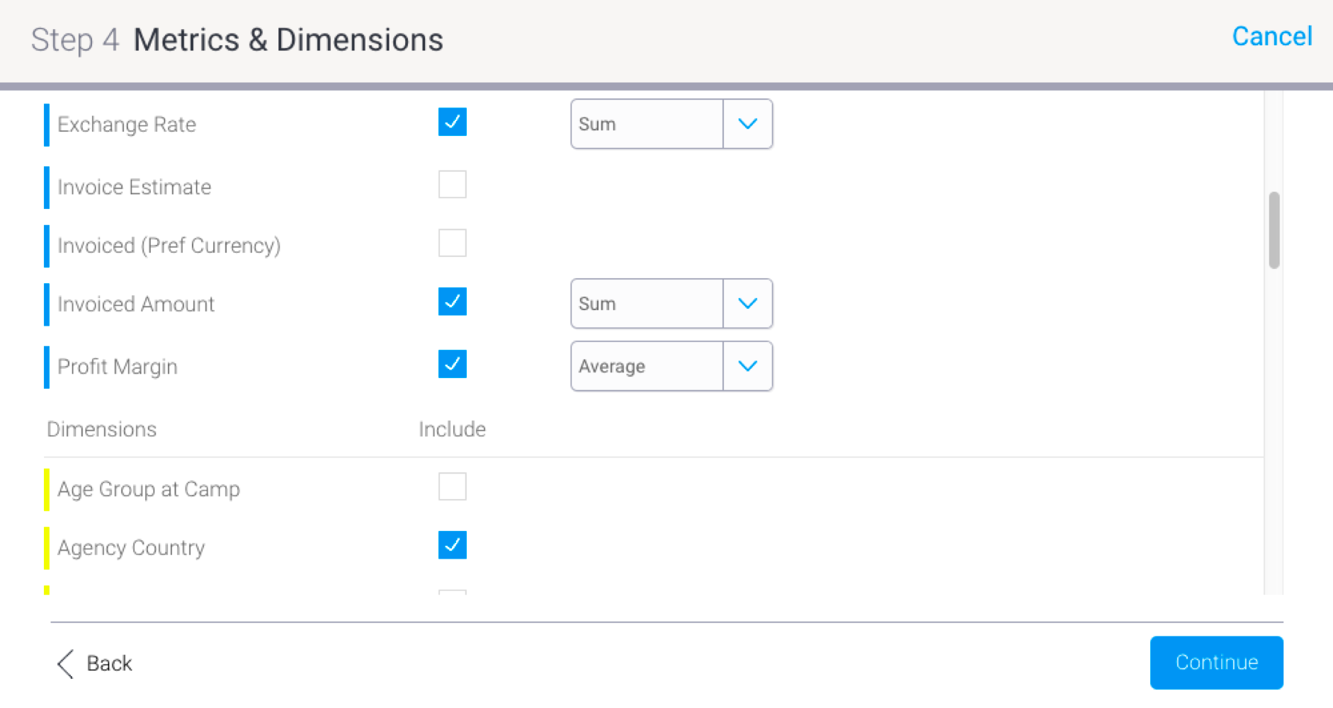
- Metrics: Choose the numeric fields that will be analyzed, such as age, sales, profit. A default aggregation type must be specified for each metric for it to be analyzed. Choose one of the following aggregation types:
Note: Choosing the right aggregation type for the metric is important. For example, instead of observing the sum of the Internet speed over time, it would be ideal to look at the average value of this metric. Some metrics will can be summed or averaged. This selection will affect the Signals that are generated.- Sum: generates insights based on the sum or total of the selected metric field.
- Average: generates insights based on the average of the selected metric field.
- Dimensions: Select the dimension fields that are relevant to the analysis. The system will look for Signals related to these fields. (Note: Selecting too many may slow down the analysis.)
- Metrics: Choose the numeric fields that will be analyzed, such as age, sales, profit. A default aggregation type must be specified for each metric for it to be analyzed. Choose one of the following aggregation types:
- Proceed to the next step by clicking on the Continue button.
- In the Algorithm Parameters step, you can configure advanced Signals settings. These configurations will be specific to the selected analysis type, and the algorithms involved. See below for explanation on these.
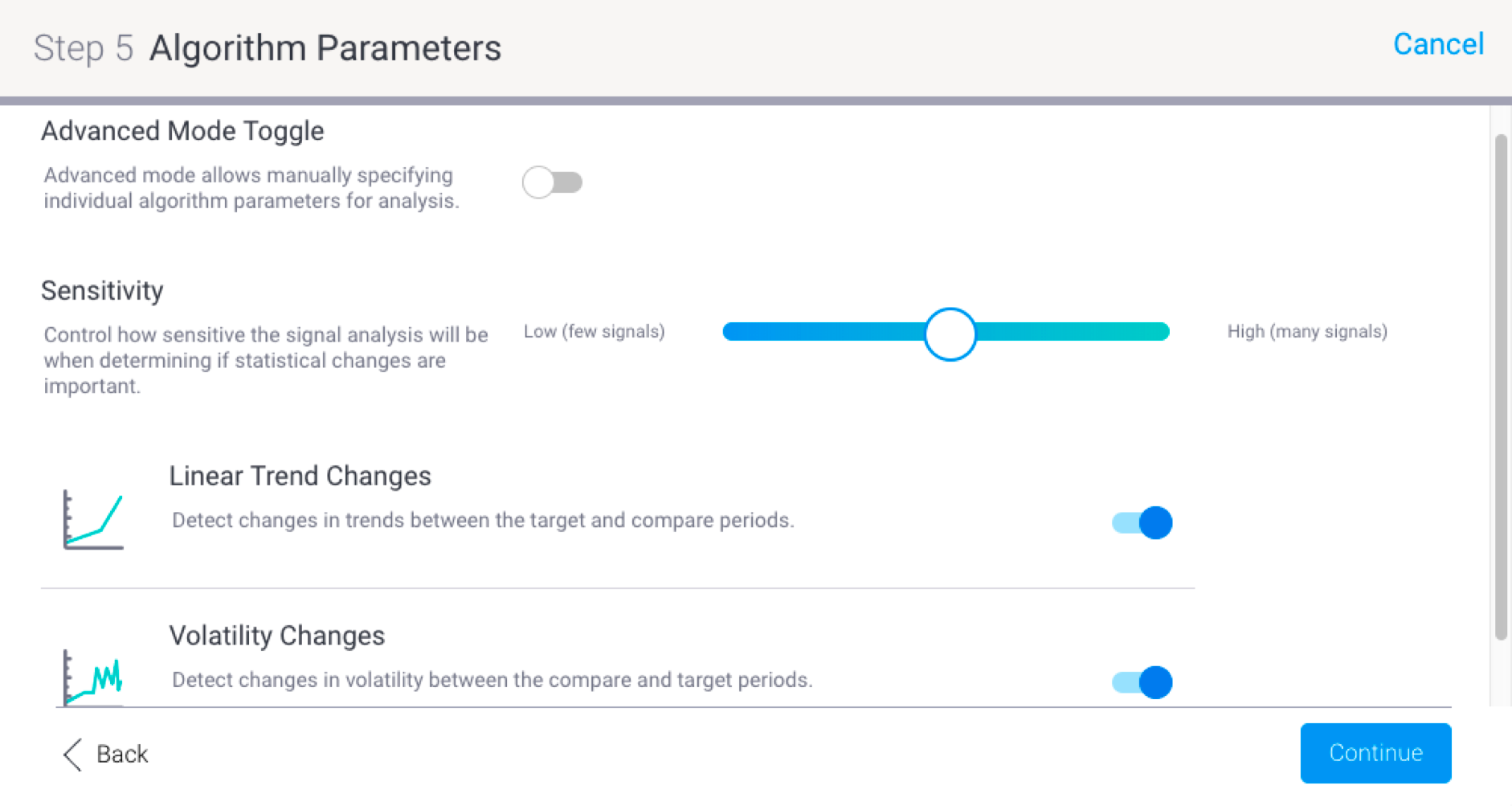
- Configure sensitivity: Signals are generated when a detected data event exceeds pre-defined threshold. Use this slider to automatically increase or decrease these thresholds. The higher the sensitivity, the more signals will be generated.
- Advanced mode toggle: Use this toggle to view additional advanced settings. Descriptions for these are below, depending on the selected analysis group.
Maximum alerts: You can set a limit to the number of alerts that are generated each time a Signals analysis is run.
Advanced parameters for Outliers analysis:Parameter
Description
Example
Spikes, drops, and steps

This algorithm looks for sudden increases (steps) or decreases (drops) in metric value. If successive Steps or Drops are detected, they are reported as a Step Up or Step Down respectively, signifying that there has been a breakout.
Use this toggle to enable this algorithm and bring up additional configuration options related to it.
Example of a spike, a lot of extra website visits occurred on a specific day.
Lag
Specify a numeric value as lag to calculate the moving average. It affects how slowly the moving average will reflect the changes in the time series trend. The higher the lag, the smoother will be the moving average, which will be more tolerant to erratic data.
This value should be lower than the number of data points in each analysis period to generate a signal.
Note: The minimum value of 3 is required for the lag, no lower than that.
A typical value of 10% of the data might generate signals.
For a month (with roughly 30 days) worth of daily data, use a lag of 3 (or higher).
Influence
Define a numeric value between 0 and 1 which controls how strongly an outlier will impact the moving average. A high influence value will cause the moving average to more closely follow the time series.
A typical value for influence is 0.3.
Threshold
Specifies the moving average corridor size in standard deviations. A higher value causes the corridor to be larger, requiring a larger magnitude of change to detect an outlier.
This value defines the width of the border used to detect outliers. A high value will mean that outliers detected above it will be identified, resulting in big anomaly detection.
A typical value of 3.5 to 4.5 should detect significant outliers.
Advanced configuration for Period Comparison:Parameter
Description
Example
Aggregate value changes
This algorithm detects changes in sum and average value of a metric from one period to another.
Use this toggle to enable this algorithm and bring up additional configuration options related to it. See below.
Eg. Total sales amount has dropped significantly this month compared to last month.
Sum aggregates
This algorithm detects changes in the total value of the metric field.
Use this toggle to enable this algorithm.
Threshold %
A change in total must have an absolute percentage greater than this threshold to constitute a signal.
For example, a threshold of 10 will result in any sum changes greater than 10% being created as Signals.
Threshold Absolute
A change in sum must have an absolute value greater than this threshold to constitute a signal.
For example, a value of 20 will consider any sum changes greater than 20 as a signal.
Average aggregates
This algorithm detects changes in the average of a metric field.
Use this toggle to enable this algorithm.
Threshold %
A change in average must have an absolute percentage greater than this threshold to constitute a signal.
For example, a threshold of 10 will result in any average changes greater than 10% being created as Signals.
Threshold Absolute
A change in average must have an absolute value greater than this threshold to constitute a signal.
For example, a value of 20 will classify any average changes greater than 20 as a signal.
New and lost attributes
This algorithm detects key dimensions that entered or left the data this period.
Use this toggle to enable this algorithm and bring up additional configuration options related to it. See below
Eg. A customer that bought a lot last month stopped buying this month.
Minimum significance
A new or lost attribute's total series percentage must be greater than this threshold to constitute a signal.
A minimum significance value of 20% would mean an attribute must make up more than 20% of total data to be detected as a signal.
Advanced parameters for Trend Changes:Parameter
Description
Example
Linear Trend Changes
This algorithm detects changes in trend line slopes from one period to another, such as trend going from up to down, or growing significantly faster or slower.
Use this toggle to enable the algorithm, and configure settings related to it.
PC sales were growing but started to decline last month.
Threshold %
A change in trend slope must have an absolute percentage greater than this threshold to constitute a signal.
For eg, a value of 10 will result in any trend slope change greater than 10% being created as Signals.
Threshold absolute
A change in trend slope must have an absolute value greater than this threshold to constitute a signal.
For example, a value of 20 will consider any trend slope change value greater than 20 as a signal.
Flat tolerance
This numerical value will form a range about zero (that is, the same value in -/+ range) and any trends which have a slope falling inside this range will be considered to be flat.
Values falling out of this range will be considered as having a positive slope (if a positive value), or a negative slope (that is the trend is going down because of a negative value).
For example, a flat tolerance of 0.01 means that if a trend line slope falls within -0.01 to 0.01 then it will be considered to be flat.
Volatility changes
Detect changes in volatility between the compare and target periods. Measures changes in consistency of metric values.
Use this toggle to enable the algorithm, and configure settings related to it.
Eg. Daily sales of Blue Shoes was sporadic last month, but has become more regular.
Threshold %
A change in volatility must have an absolute percentage greater than this threshold to constitute a signal.
For example, a threshold % of 10 will result in any volatility changes greater than 10% to be classified as a Signal.
Threshold absolute
A change in volatility must have an absolute value greater than this threshold to constitute a signal.
For example, a value of 20 will classify any volatility changes greater than 20 as a signal.
Continue to the next step.
- In the Access step, you can select users who’s related data will be included in the analysis (by default every user’s data will be included in the analysis, but we can choose to include only specific users here).
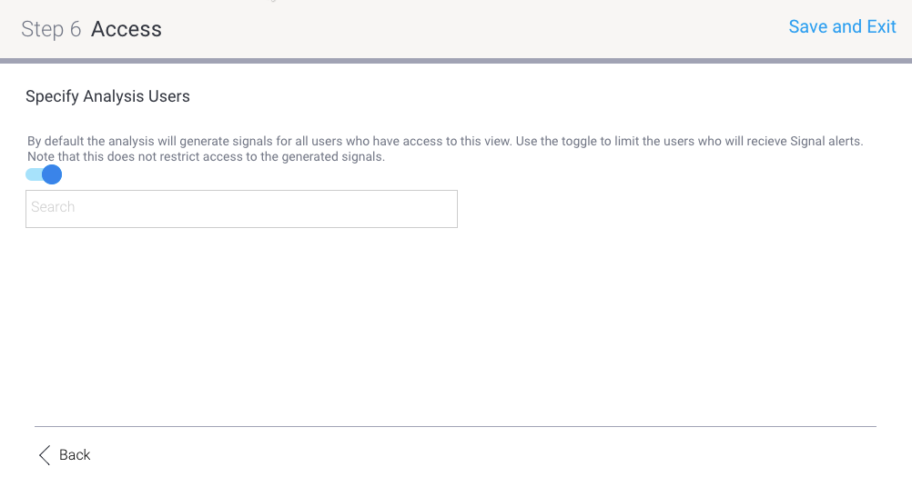
- Enable the toggle to include users in this analysis schedule.
- Then search and select these users (or groups).
- Once all the configurations are provided, save this analysis by clicking on the Save and Exit button in the top corner.

- The saved Signals analysis will appear in the list. You can delete an analysis or copy it to create a new one.

- To edit an analysis, click on its name.
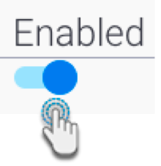
- Use the Enabled toggle to enable or disable an analysis. Disabling it would stop it from generating or detecting Signals.
- Click Submit once done.
- Exit the view builder. Note: it is not mandatory to save your View after creating a Signals analysis.
- The Signals analysis will run according to schedule. However, to manually run an analysis, refer to the section below.
...