Page History

...

1. To set up a Signals analysis, navigate to the main Signals page. (Left side navigation > Signals)
   
   
   
   
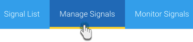
2. Click on the Manage Signals tab.
   
   
   
   

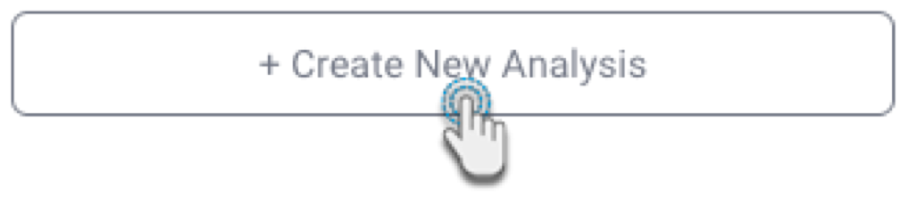
3. Click on the +Create New Analysis button to create a new Signals analysis. This initiates a multi-step configuration process to help you set up the automated analysis relevant to you.

   

   
   
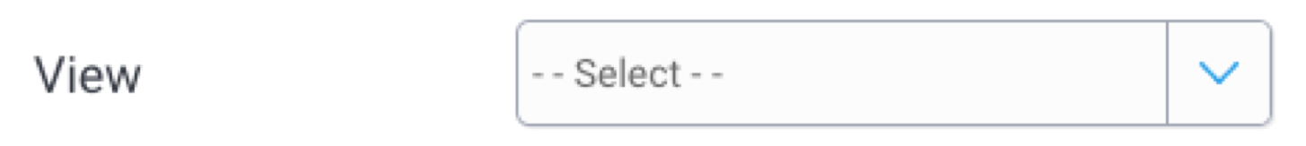
   Step 1: Analysis group type
   
   

4. Select the relevant View. The data of this View will be auto-analyzed by the system.
   
   
   
   

5. Establish the type of analysis that you want the system to perform for you. There are three analysis types to choose from. (Refer to the Signal types section to identify which type of anomaly to detect through one of these analysis types.)
   
   
   
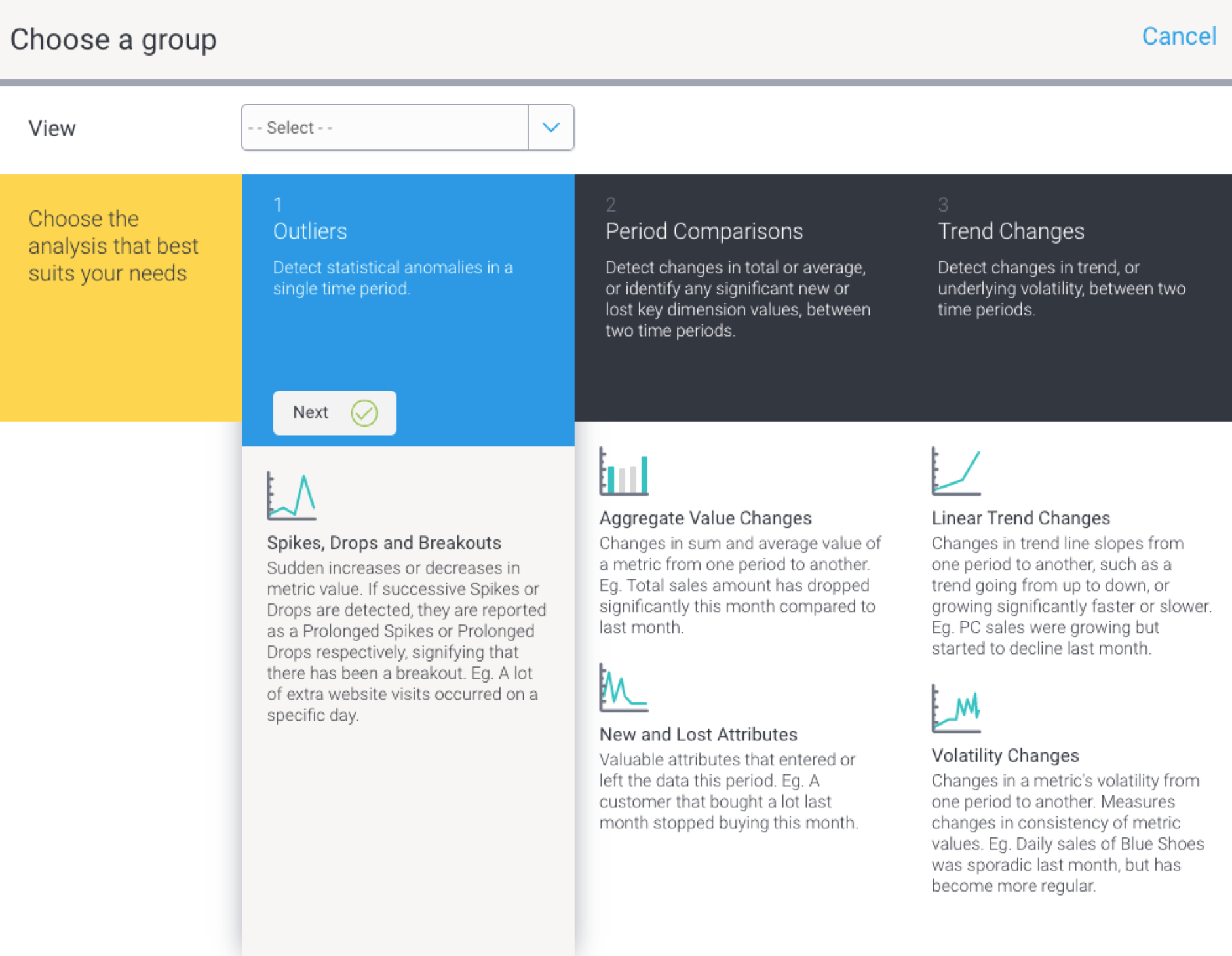
   Here's a quick overview of each analysis group:

   Analysis Group	Description
   Outliers	The system detects any anomalies in the data, such as spikes/drops and breakouts during a specific time window. These could include rare events, items or observations that are significantly different from the majority of the data.
   Period comparisons	Identifies changes in total or average between two time periods; and also identifies any significant new or lost key dimension values.
   Trend changes	Identifies changes in trend direction between two time periods; and also any changes in the underlying volatility of the data.

   
   
   

6. Click on the Next button of the preferred analysis to continue.

   

   
   Step 2: Name and description
   
   

7. In this step, provide the basic details to describe this analysis.
   
   
   
   

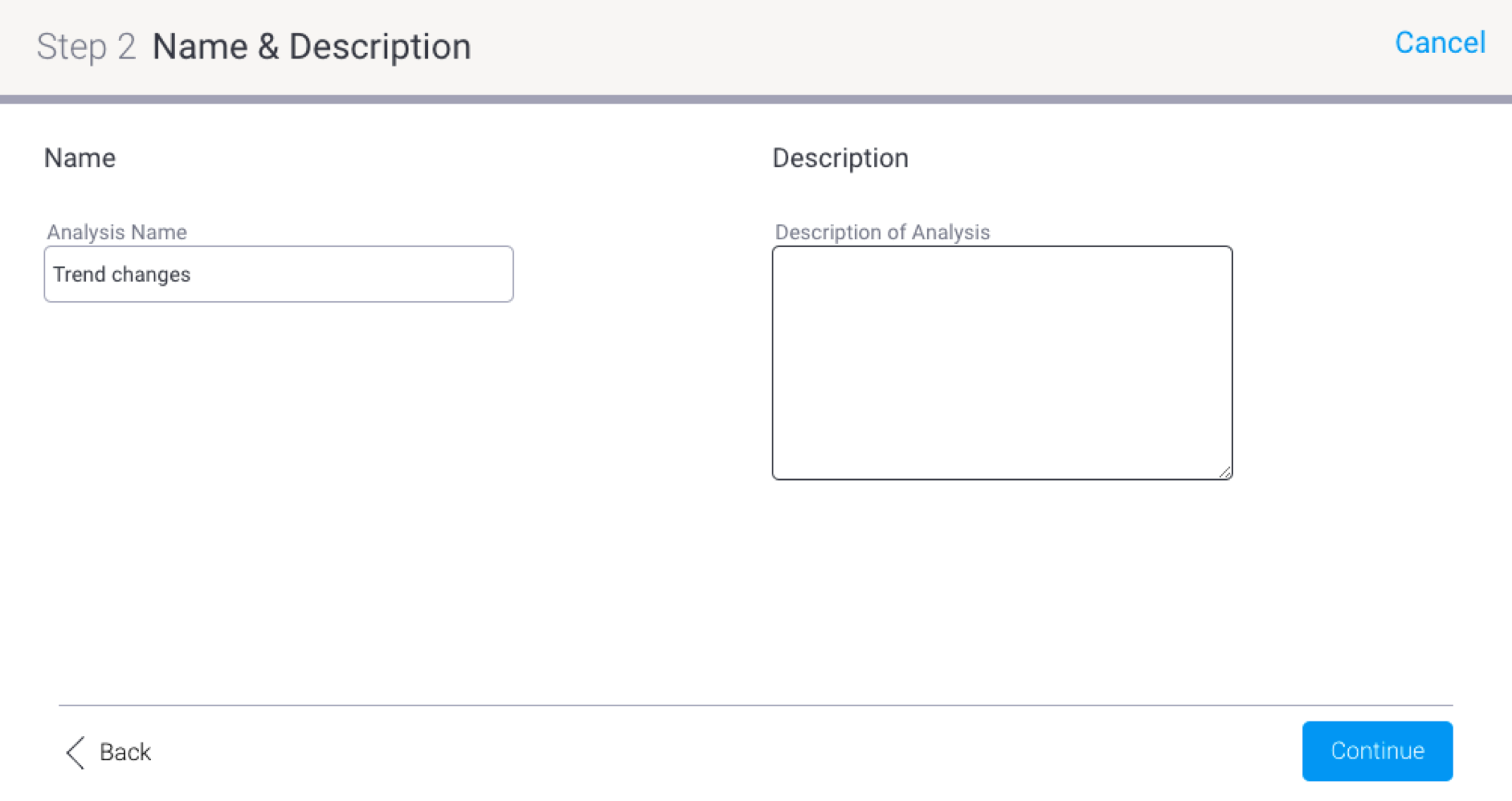
   1. Analysis Name: (mandatory field) A unique name will help you to identify it later.
   2. Description of Analysis: Add a description to explain the intent of this analysis.

8. Continue to the next step.

   
   

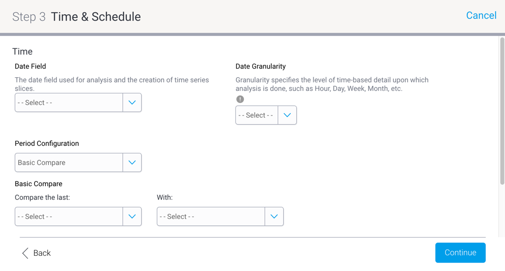
   Step 3: Time & schedule

   
   

9. The Time & Schedule step involves highlighting the time periods that you want the system to analyze, along with configuring how frequently this analysis should be executed. Below is a description of each of the settings. (Note: The fields and their purpose differ according to the different analysis types.)
   
   
   
   

   Field	Analysis type	Description	Example
   Date field	All	The Signal analysis must include a date field that gets analyzed by the system. This is required to form a time series. You can choose a date field of any granularity (unit).
   Date Granularity	All	Specify the granularity (i.e. date unit) of the time series to analyze. This value should not be lower than the unit of your selected date field.	For example, if you have a date field with day, then your granularity must be Day or a higher value (Month, Quarter, etc.)
   Period Configuration	All	This selection changes the time window selection fields. Options are: Basic compare: Provides basic options to select time periods. Advanced compare: Brings up advanced options for configuring the time period, that is, Window Size, and Offset. Fixed Range: To select an exact date range. Useful when running one-off Signals analysis. Note: For Outlier analysis, only a single time period needs to be specified.
   Basic compare fields
   Compare the last	All	Specify the main time period window to be analyzed.	Analyze the last ‘month’ will simply analyze the previous month.
   With	Only Period compare and Trend changes	Specify a secondary time period to be analysed. This time period is compared to the main target period specified above.	Based on the above example, if this field was set to ‘quarter’, then the previous month will be compared and analyzed with the same month from the last quarter. (So the third month of the last quarter will be compared to the third month of the previous quarter.)
   Advanced compare fields
   Window size	All	This advanced configuration specifies the length of the time period to be analyzed. The value of the selected unit will always be 1. In case of period compare and trend changes where two time periods are analyzed, both the time periods will be of the same length.	A window size of 1 month will analyze the last month for Outlier detection; or compare the last month, with the previous month prior to that, for Period comparision or Trend Changes.
   Offset	Period comparison	Use this advanced field to specify a time distance between the two time periods. A distance of the size specified here is formed from the end of the previous period to the beginning of the current period. An offset of 1 creates two sequential periods. Cannot have value of 0 as an offset.	Say your window size is 3 months (from 1st Jan to 31st Mar 2018), an offset of 11 months, will compare the same 3 months (1st Jan to 31st Mar) of the previous year, i.e. 2017. Or if offset is set to 1, compare the last 3 months with previous 3 months.
   	Trend changes	Use this advanced field to specify a time distance between the two time periods. A distance of the size specified here is formed from the end of the previous period to the end of the current period. An offset of 1 window size unit creates two sequential periods. Cannot have value of 0 as an offset.	For a window size of 3 months, where the offset is set to 1 year, the last 3 months are compared to 3 months from a year ago.
   	Outliers	Specifies how long ago should the target window size be analyzed. Cannot have value of 0 as an offset.	If window size is 3 weeks, and offset is 5 months, then analyze 3 weeks from 5 months ago.
   Fixed range fields
   Target Period	All	Specify a fixed date range to analyze using the date picker
   Compare period	Only period compare, trend analysis	If your selected analysis compares two time periods, then specify the other one here. Note that the target period must be after the compare period. Both the periods should be of similar length.
   Schedule fields
   Schedule	All	Set a schedule for when and how frequently this analysis job should run. Note: For a weekly frequency or higher, use the Advanced Setting link for further specification.	You can schedule your analysis to automatically run every Monday at noon, for example.
   Frequency	All	Depending on the option selected here, you may be required to provide further details. Tip: Select 'Once' as the frequency to send out the broadcast as soon as possible.	For example, if Fortnightly is selected, you will be prompted to select either the first or second week of the fortnight to send in, as well as the day of the week.
   Timezone	All	Sometimes you may find you need to set the Time Zone, and local time for delivery. This can be accomplished by clicking the Advanced Settings link.

   
   

10. Continue to the next step to proceed.

    
    

    Step 4: Metric & dimensions

11. In the Metrics & Dimensions step, you can select or unselect the fields in your data, that are important to you. Yellowfin will analyze these fields in order to detect Signals.
    
    

    Note
    Fields that are also selected for Assisted Insights, will be selected here by default. You can change these, as discusses in the additional setup process below.

    
    
    
    

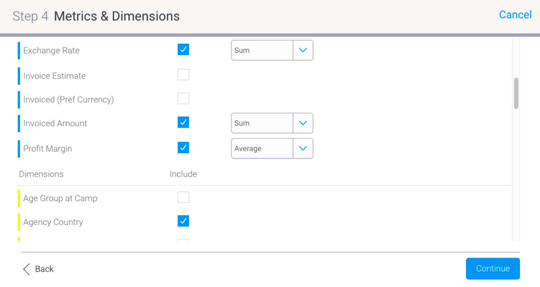
    1. Metrics: Choose the numeric fields that will be analyzed, such as age, sales, profit. A default aggregation type must be specified for each metric for it to be analyzed. Choose one of the following aggregation types:
       
       

       Tip

       Choosing the right aggregation type for the metric is important. For example, instead of observing the sum of the Internet speed over time, it would be ideal to look at the average value of this metric. Some metrics will can be summed or averaged. This selection will affect the Signals that are generated. The aggregation will be preselected if the field already has one applied, however you can change it (unless it’s a specific type of calculated field). If no aggregation is preselected, then Sum would be chosen by default.

       
       

       • Sum: generates insights based on the sum or total of the selected metric field.

       • Average: generates insights based on the average of the selected metric field.
         
         

         Calculated fields are also supported, but their aggregation cannot be changed. This affects the Signal narrative as the aggregation type will not be mentioned in it. There are, however, certain cases of calculated field that aren’t supported in the Signals analysis: this includes those with average aggregation, or calculation containing a dynamic ratio (meaning a ratio that involves two fields). If such a field is selected, it will bring up a warning message.
         
         
         

    2. Dimensions: Select the dimension fields that are relevant to the analysis. The system will look for Signals related to these fields. (Note: Selecting too many may slow down the analysis.)
12. Proceed to the next step by clicking on the Continue button.
    
    

    Step 5: Filters

13. The Filter step is used to add conditional filters on your View data. If your View contains a vast range of data, you may not want to include all the data in the analysis. This allows you to control the data that you want the Signals engine to focus on.
    Note: The filter condition will become the ‘baseline’ of the Signals.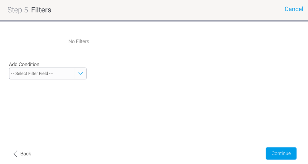
    
    
    
    

14. To create a filter condition, ensure that you understand the above screen.
    
    

    Expand
    title Expand this to understand the filter screen...
    Section Column width 50 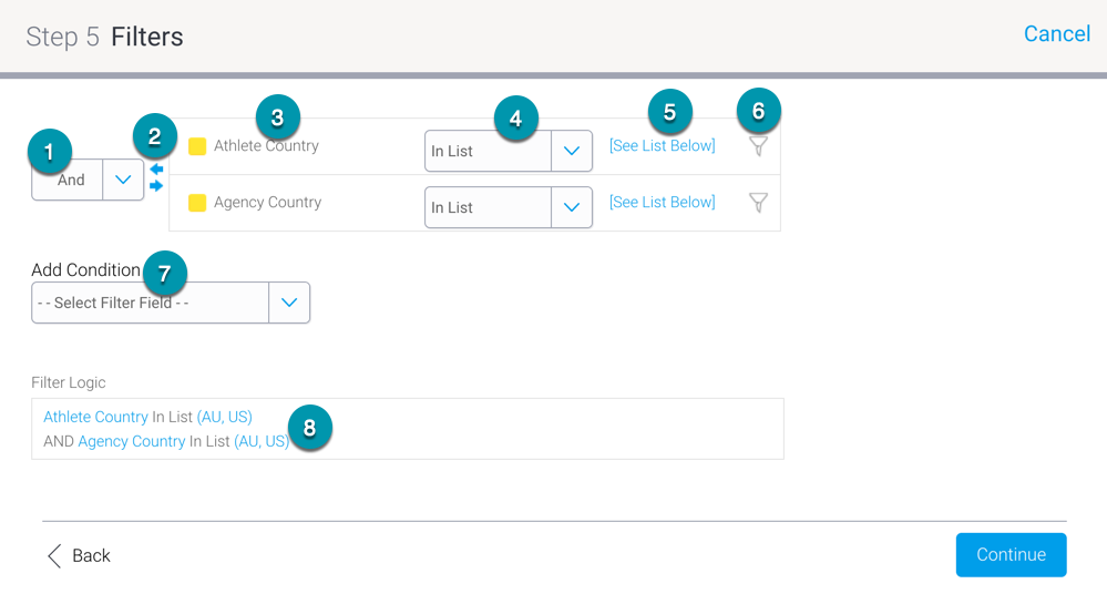Column width 50 No. Filter Setting Description 1 AND/OR Logic Define the logic used between each filter condition. Appears in case of multiple conditions. 2 Bracket Arrows The addition of brackets around sets of filters allows for more complex logic, used in conjunction with AND/OR logic settings. 3 Filter Fields The fields added to the Filters list in order to restrict the Signal results. 4 Operator  Select the operator to be used in the filter, specifying how values will need to match, or differ from the condition defined. 5 Value Selection Define a value for the filter condition. 6 Value Search Brings up a selection popup to search for and add values. 7 Add Condition Allows the user to add more fields to the filters list in the same Signal analysis. 8 Filter Logic Displays a summary of the filters.

    
    

15. Create a filter condition by choosing a field. Yellowfin filters work by establishing a condition on a field. 
16. Then specify an operator for the selected field and define the value. 
17. You can add more filter conditions by adding more fields, and doing the same for them. Then define the ADD/OR logic between the multiple conditions.
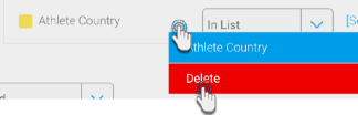
18. To delete a Signal filter, hover over the field name until the dropdown menu icon appears, then click on it and select Delete.
    
    
    
    
19. Once all the conditions are defined, proceed to the next step.
    

    
    Step 6: Algorithm parameters

20. In the Algorithm Parameters step, you can configure advanced Signals settings. These configurations will be specific to the selected analysis type, and the algorithms involved. See below for explanation on these.
    
    
    
    
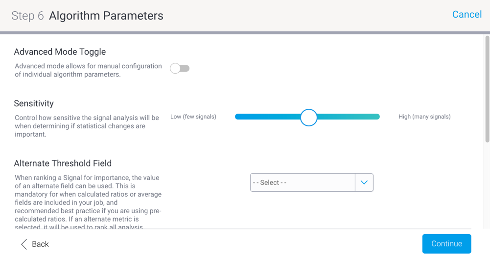
    1. Advanced mode toggle: Use this toggle to view additional advanced settings. Descriptions for these are in the tables below, according to their selected analysis group.
       
    2. Configure sensitivity: Signals are generated when a detected data event exceeds pre-defined threshold. Use this slider to automatically increase or decrease these thresholds. The higher the sensitivity, the more signals will be generated. 
    3. Enable Correlation analysis: Enable this toggle to perform correlation analysis. Tip: You can disable correlation to speed up an analysis where comparing correlated data is not required.

    4. Alternate threshold field: This parameter is specifically used for determining importance of Signals for the user base. When ranking a Signal for importance, the value of an alternate field can be used. This is mandatory for when calculated ratios or average fields are included in your job, and recommended best practice if you are using pre-calculated ratios. If an alternate metric is selected, it will be used to rank all analysis metrics in this job. Leave blank if you want to use the analysis metric to determine the threshold. 
       
       General advanced parameters:
       These are the general advanced parameters that can be configured for each analysis group. Note that their default values will differ according to the level of the Sensitivity Slider.
       
       

       Parameter	Description
       Max Timeline Signals	The users receive alerts on relevant Signals in their Timeline. This parameter is used to define the maximum number of alerts that will be delivered to their Timeline. If more Signals are generated than this limit, they will be available in the user's Signal list.
       Max Correlated Signals Displayed	The Signals engine looks at all of your data (in different views and databases) to see if there are data patterns similar to the current time series. This lets you know of possible relationships in your business, even if the matching patterns in data are not from the same data set, not even the same metrics or dimensions. We call this Correlation. The correlation lines will appear in the Signal detail page to let you compare and explore these relationships in data. There could be a large number of these lines. Use this to specify the maximum number of the most matching correlated lines that will appear in the Signals UI to be compared with the time series line.
       Min Correlated Threshold	Correlation between 2 lines is calculated in a range of -1 to 1, where -1 signifies that the lines are moving in opposite directions, and +1 signifies that they’re going in the same direction. However, a value of 0 or very close to it means there’s no correlation. This threshold lets you alter this range for 0, so if the threshold is 0.4, then correlation ranging from -1 to -0.4 and 0.4 to 1 will be detected.
       Analysis Threshold %	This threshold eliminates Signals that are of low value to the user. Only the total value of time slices that are equal to or greater than the defined % of the total baseline value will be considered important enough to analyse. For example, if your threshold is 2% and your baseline metric is Total Sales for Europe ($100,000) then Sales for Germany ($10,000 or 10% of baseline) or any country above $2000, will be analysed but Sales for Poland ($1,000 or 1% of baseline) or any country below will not. Generally values below 1% are best, with a maximum of 25%.
       Alternate Threshold Field	This parameter is specifically used for determining the importance of Signals for the user base. When ranking a Signal for importance, the value of an alternate field can be used. This is mandatory for when calculated ratios or average fields are included in your job, and recommended best practice if you are using pre-calculated ratios. If an alternate metric is selected, it will be used to rank all analysis metrics in this job. Leave blank if you want to use the analysis metric to determine the threshold.

       
       
       Advanced parameters for Outliers analysis:

       Parameter	Description	Example
       Spikes, drops, and breakouts	This algorithm looks for sudden increases (steps) or decreases (drops) in metric value. If successive Steps or Drops are detected, they are reported as a Prolonged Steps or Prolonged Drops respectively, signifying that there has been a breakout. Use this toggle to enable this algorithm and bring up additional configuration options related to it.	Example of a spike, a lot of extra website visits occurred on a specific day.
       Baseline Period	The baseline period is the number of date time periods used to create a moving average used in the analysis period. The longer the baseline, the smoother the moving average. The baseline period is recommended to be at least 1 seasonality cycle long. However, very long baseline periods will affect how long the signal job needs to run as more data is analysed.
       Baseline Outlier Influence on Moving Average	Outliers in the baseline period can influence the detection of Outliers in the analysis period by affecting the moving average and standard deviations. Use this setting to reduce its impact.  Important: This value should be larger than 0, as a value equal or close to 0 may lead to zero confidence interval. If the confidence interval is zero, all values not equal to the moving average will be regarded as a Signal.	A 30% reduction of outlier value is considered reasonable.
       Confidence Range Width	The confidence interval or range is the value above or below the moving average that is considered normal. Outliers are values that sit outside of the confidence range. Use this setting to specify the range width in standard deviations from the moving average. A higher value makes the range larger, requiring a bigger spike or drop to be recognised as an outlier.	This value must be between 2 and 5 with 3 being a reasonable setting.
       Use Seasonality	Enable toggle to detect and use seasonality when identifying outliers and breakouts. Seasonality refers to a repeating pattern in a time series.  Tip: If these repeating patterns are expected behaviour, and you do not want Signals generated for this, you can disable this toggle.	For e.g. sale spikes occurring every Christmas will be a seasonal pattern.
       Automatically detect periodicity	Periodicity is a time series concept that determines the length of time period between seasonal patterns.  If enabled, Yellowfin will try to detect the periodical pattern in your data automatically. Otherwise, you will need to provide the periodicity explicitly.  If no valid periodical pattern is auto detected, Yellowfin will not use seasonality when identifying outliers.	Based on the above Christmas example, the periodicity will be a year (every Christmas).
       Data Periodicity	If automatic periodicity detection is disabled, use this parameter to explicitly provide periodicity that you would like to use in seasonality.  Note: Periodicity is mandatory to be specified when seasonality is enabled, and the above configuration is disabled. You must specify a value bigger than 3 for seasonality analysis to work.	Tip: The unit for date values depends on your specified date granularity. So if your selected granularity is months, then you may enter 12 to signify a year, or if it’s quarter, then 4 to get the same value.
       Old Signal Notifications	Restrict older Signals from being delivered as notifications. Older Signals refer to Signals that occurred before the last analysis was run. Enabling this results in these Signals surfacing again on Signals List, but without notifying users.
       Ignore Old Signals	Restrict older Signals from being generated. Older Signals refer to the Signals that occurred before the last analysis was run.

       
       Advanced configuration for Period Comparison:

       Parameter	Description	Example
       Aggregate value changes	This algorithm detects changes in sum and average value of a metric from one period to another. Use this toggle to enable this algorithm and bring up additional configuration options related to it.	Eg. Total sales amount has dropped significantly this month compared to last month.
       Sum aggregates	This algorithm detects changes in the total value of the metric field. Use this toggle to enable this algorithm.
       Threshold %	A change in total must have an absolute percentage greater than this threshold to constitute a signal.	For example, a  threshold of 10 will result in any sum changes greater than 10% being created as Signals.
       Threshold	A change in sum must have an absolute value greater than this threshold to constitute a signal. Note: Only of the two threshold fields can be used to specify a limit.	For example, a value of 20 will consider any sum changes greater than 20 as a signal.
       Average aggregates	This algorithm detects changes in the average of a metric field. Use this toggle to enable this algorithm.
       Threshold %	A change in average must have an absolute percentage greater than this threshold to constitute a signal.	For example, a  threshold of 10 will result in any average changes greater than 10% being created as Signals.
       Threshold	A change in average must have an absolute value greater than this threshold to constitute a signal. Note: Only of the two threshold fields can be used to specify a limit.	For example, a value of 20 will classify any average changes greater than 20 as a signal.
       New and lost attributes	This algorithm detects key dimensions that entered or left the data this period. Use this toggle to enable this algorithm and bring up additional configuration options related to it.	Eg. A customer that bought a lot last month stopped buying this month.
       Minimum significance %	A new or lost attribute's series contribution must be greater than this threshold to constitute a signal. That is, when detecting if an attribute’s contribution to the series is significant enough to qualify as a signal, its contribution percentage is compared with this setting; if it’s greater than this value, it’s a signal.	A minimum significance value of 20% would mean an attribute must make up more than 20% of total data to be detected as a signal.
       Maximum Insignificance %	A new or lost attribute's series contribution must be less than this threshold to constitute a signal. That is, when detecting if an attribute’s contribution to the series is significant enough to qualify as a signal, its contribution percentage is compared with this setting; if it’s less than this value, it’s a signal. Attributes with contributions that are too small for Min Significance, and too big for Max Insignificance, do not qualify as a signal.	A maximum insignificance value of 1% would mean an attribute must make up less than 1% of total data to be detected as a signal.

       
       Advanced parameters for Trend Changes:
       

       Parameter	Description	Example
       Linear Trend Changes	This algorithm detects changes in trend line slopes from one period to another, such as trend going from up to down, or growing significantly faster or slower. Use this toggle to enable the algorithm, and configure settings related to it.	PC sales were growing but started to decline last month.
       Threshold %	A change in trend slope must have an absolute percentage greater than this threshold to constitute a signal.	For eg, a value of 10 will result in any trend slope change greater than 10% being created as Signals.
       Threshold	A change in trend slope must have an absolute value greater than this threshold to constitute a signal. Note: Only of the two threshold fields can be used to specify a limit.	For example, a value of 20 will consider any trend slope change value greater than 20 as a signal.
       Flat Trend Gradient Tolerance	This numerical value will form a range about zero (that is, the same value in -/+ range) and any trends which have a slope falling inside this range will be considered to be flat. Values falling out of this range will be considered as having a positive slope (if a positive value), or a negative slope (that is the trend is going down because of a negative value). Note: When looking for trend changes, if the data shows a sign change (that is, it goes from a positive value or negative, or vice versa) then that always generates a Signal.	For example, a flat tolerance of 0.01 means that if a trend line slope falls within -0.01 to 0.01 then it will be considered to be flat.
       Volatility changes	Detect changes in volatility between the compare and target periods. Measures changes in consistency of metric values. Use this toggle to enable the algorithm, and configure settings related to it.	Eg. Daily sales of Blue Shoes was sporadic last month, but has become more regular.
       Threshold %	A change in volatility must have an absolute percentage greater than this threshold to constitute a signal.	For example, a  threshold % of 10 will result in any volatility changes greater than 10% to be classified as a Signal.
       Threshold	A change in volatility must have an absolute value greater than this threshold to constitute a signal. Note: Only of the two threshold fields can be used to specify a limit.	For example, a value of 20 will classify any volatility changes greater than 20 as a signal.

       
       

21. Continue to the next step.

    Anchor
    clientorg clientorg

    Step 7: Client Organizations

    
    

22. If you have a multi-client organization setup for your Yellowfin instance, then the additional Client Organizations step can be configured. Here you can choose to limit specific client organizations if you don’t want them included in the analysis (because unless specified, the system includes all the organizations by default).
    
    If enabled, the engine will only look at client organizations that can access the View this analysis is created in. (Note, however, that users of disabled organizations will still be able to access previously generated Signals, if the client orgs already exist. But if they’re new, they will not be able to access the Signals.)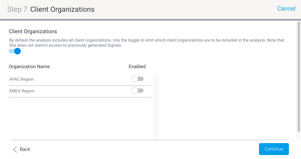
    
    
    
    

    1. Enable the main toggle to initiate the client organization limitation functionality. A list of all your client orgs will appear.

    2. Enable the toggle for any client organization that you do want to include the analysis. (Clients with disabled toggles will not be included.)

    3. If you want to exclude all client organizations, leave their toggles disabled.

23. Continue to the next step.
    
    

    Step 8: Users

    
    

24. In the Users step, you can select users whose related data will be included in the analysis (by default every user’s data will be included in the analysis, but we can choose to include only specific users here).
    
    
    
    
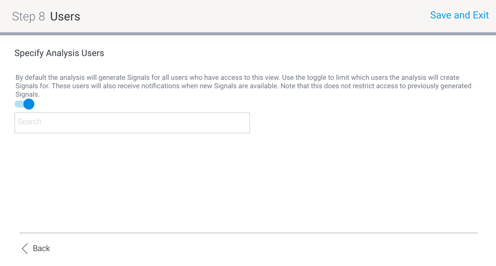
    1. Enable the toggle to include users in this analysis schedule.
    2. Then search and select these users (or groups).
       
       
25. Once all the configurations are provided, save this analysis job by clicking on the Save and Exit button in the top corner.
    
    
    
    
26. The saved Signals analysis job will appear in the list. Learn more about managing these analysis jobs here. 
27. Click Submit once done.
28. Publish the view, and exit the view builder.
29. The Signals analysis will run according to schedule. However, to manually run an analysis, refer to the section below.
    
    

...